VI Accumulators
When you ask ISL+ to apply some function f to an argument a, you usually get some value v. If you evaluate (f a) again, you get v again. As a matter of fact, you get v no matter how often you request the evaluation of (f a).The function application may also loop forever or signal an error, but we ignore these possibilities. We also ignore random, which is the true exception to this rule. Whether the function is applied for the first time or the hundredth time, whether the application is located in DrRacket’s interactions area or inside the function itself, doesn’t matter. The function works according to its purpose statement, and that’s all you need to know.
This principle of context-independence plays a critical role in the design
of recursive functions. When it comes to design, you are free to assume
that the function computes what the purpose statement promises—
While context-independence facilitates the design of functions, it causes two problems. In general, context-independence induces a loss of knowledge during a recursive evaluation; a function does not “know” whether it is called on a complete list or on a piece of that list. For structurally recursive programs, this loss of knowledge means that they may have to traverse data more than once, inducing a performance cost. For functions that employ generative recursion, the loss means that the function may not be able to compute the result at all. The preceding part illustrates this second problem with a graph traversal function that cannot find a path between two nodes for a circular graph.
This part introduces a variant of the design recipes to address this “loss of context” problem. Since we wish to retain the principle that (f a) returns the same result no matter how often or where it is evaluated, the only solution is to add an argument that represents the context of the function call. We call this additional argument an accumulator. During the traversal of data, the recursive calls continue to receive regular arguments while accumulators change in relation to those and the context.
Designing functions with accumulators correctly is clearly more complex than any of the design approaches from the preceding chapters. The key is to understand the relationship between the proper arguments and the accumulators. The following chapters explain how to design functions with accumulators and how they work.
31 The Loss of Knowledge
Both functions designed according to structural recipes and the generative
one suffer from the loss of knowledge, though in different ways. This
chapter explains with two examples—
31.1 A Problem with Structural Processing
Let’s start with a seemingly straightforward example:
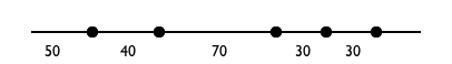
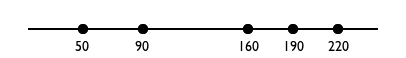
Sample Problem You are working for a geometer team that will measure the length of road segments. The team asked you to design a program that translates these relative distances between a series of road points into absolute distances from some starting point.
Designing a program that performs this calculation is a mere
exercise in structural function design. Figure 177
contains the complete program. When the given list is not '(),
the natural recursion computes the absolute distance of the remainder of
the dots to the first one on (rest l). Because the first
is not the actual origin and has a distance of (first l) to the
origin, we must add (first l) to each number on the result of
the natural recursion. This second step—
; [List-of Number] -> [List-of Number] ; converts a list of relative to absolute distances ; the first number represents the distance to the origin (check-expect (relative->absolute '(50 40 70 30 30)) '(50 90 160 190 220)) (define (relative->absolute l) (cond [(empty? l) '()] [else (local ((define rest-of-l (relative->absolute (rest l))) (define adjusted (add-to-each (first l) rest-of-l))) (cons (first l) adjusted))])) ; Number [List-of Number] -> [List-of Number] ; adds n to each number on l (check-expect (cons 50 (add-to-each 50 '(40 110 140 170))) '(50 90 160 190 220)) (define (add-to-each n l) (cond [(empty? l) '()] [else (cons (+ (first l) n) (add-to-each n (rest l)))])) Figure 177: Converting relative distances to absolute distances
(relative->absolute (build-list size add1))
size
1000
2000
3000
4000
5000
6000
7000
time
25
109
234
429
689
978
1365
Exercise 489. Reformulate add-to-each using map and lambda.
(relative->absolute (build-list size add1))
Considering the simplicity of the problem, the amount of work that the program performs is surprising. If we were to convert the same list by hand, we would tally up the total distance and just add it to the relative distances as we take steps along the line. Why can’t a program do so?
(define (relative->absolute/a l) (cond [(empty? l) ...] [else (... (first l) ... ... (relative->absolute/a (rest l)) ...)]))
(relative->absolute/a (list 3 2 7)) == (cons ... 3 ... (relative->absolute/a (list 2 7))) == (cons ... 3 ... (cons ... 2 ... (relative->absolute/a (list 7)))) == (cons ... 3 ... (cons ... 2 ... (cons ... 7 ... (relative->absolute/a '()))))
Again, the problem is that recursive functions are independent of their context. A function processes L in (cons N L) the same way as in (cons K L). Indeed, if given L by itself, it would also process the list in that way.
To make up for the loss of “knowledge,” we equip the function with an additional parameter: accu-dist. The latter represents the accumulated distance, which is the tally that we keep when we convert a list of relative distances to a list of absolute distances. Its initial value must be 0. As the function traverses the list, it must add its numbers to the tally.
(define (relative->absolute/a l accu-dist) (cond [(empty? l) '()] [else (local ((define tally (+ (first l) accu-dist))) (cons tally (relative->absolute/a (rest l) tally)))]))
(relative->absolute/a (list 3 2 7)) == (relative->absolute/a (list 3 2 7) 0) == (cons 3 (relative->absolute/a (list 2 7) 3)) == (cons 3 (cons 5 (relative->absolute/a (list 7) 5))) == (cons 3 (cons 5 (cons 12 ???))) == (cons 3 (cons 5 (cons 12 '())))
The hand-evaluation shows just how much the use of an accumulator simplifies the conversion process. Each item in the list is processed once. When relative->absolute/a reaches the end of the argument list, the result is completely determined and no further work is needed. In general, the function performs on the order of N natural recursion steps for a list with N items.
One problem is that, unlike relative->absolute, the new function consumes two arguments, not just one. Worse, someone might accidentally misuse relative->absolute/a by applying it to a list of numbers and a number that isn’t 0. We can solve both problems with a function definition that uses a local definition to encapsulate relative->absolute/a; figure 178 shows the result. Now, relative->absolute is indistinguishable from relative->absolute.v2 with respect to input-output.
; [List-of Number] -> [List-of Number] ; converts a list of relative to absolute distances ; the first number represents the distance to the origin (check-expect (relative->absolute.v2 '(50 40 70 30 30)) '(50 90 160 190 220)) (define (relative->absolute.v2 l0) (local ( ; [List-of Number] Number -> [List-of Number] (define (relative->absolute/a l accu-dist) (cond [(empty? l) '()] [else (local ((define accu (+ (first l) accu-dist))) (cons accu (relative->absolute/a (rest l) accu)))]))) (relative->absolute/a l0 0))) Figure 178: Converting relative distances with an accumulator
(relative->absolute.v2 (build-list size add1))
size
1000
2000
3000
4000
5000
6000
7000
time
0
0
0
0
0
1
1
(define (relative->absolute l) (reverse (foldr (lambda (f l) (cons (+ f (first l)) l)) (list (first l)) (reverse (rest l)))))
Does your friend’s solution mean there is no need for our complicated design in this motivational section? For an answer, see Recognizing the Need for an Accumulator, but reflect on the question first. Hint Try to design reverse on your own.
31.2 A Problem with Generative Recursion
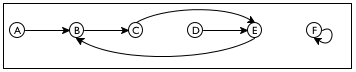
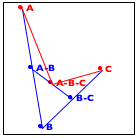
Sample Problem Design an algorithm that checks whether two nodes are connected in a simple graph. In such a graph, each node has exactly one, directional connection to another, and possibly itself.
Consider the sample graph in figure 179. There are six nodes, A through F, and six connections. A path from A to E must contain B and C. There is no path, though, from A to F or from any other node besides itself.
(define a-sg '((A B) (B C) (C E) (D E) (E B) (F F)))
; A SimpleGraph is a [List-of Connection] ; A Connection is a list of two items: ; (list Node Node) ; A Node is a Symbol.
; Node Node SimpleGraph -> Boolean ; is there a path from origin to destination ; in the simple graph sg (check-expect (path-exists? 'A 'E a-sg) #true) (check-expect (path-exists? 'A 'F a-sg) #false) (define (path-exists? origin destination sg) #false)
The problem is trivial if origin is the same as destination.
The trivial solution is #true.
If origin is not the same as destination, there is only one thing we can do: step to the immediate neighbor and search for destination from there.
There is no need to do anything if we find the solution to the new problem. If origin’s neighbor is connected to destination, then so is origin. Otherwise there is no connection.
; Node Node SimpleGraph -> Boolean ; is there a path from origin to destination in sg (check-expect (path-exists? 'A 'E a-sg) #true) (check-expect (path-exists? 'A 'F a-sg) #false) (define (path-exists? origin destination sg) (cond [(symbol=? origin destination) #t] [else (path-exists? (neighbor origin sg) destination sg)])) ; Node SimpleGraph -> Node ; determine the node that is connected to a-node in sg (check-expect (neighbor 'A a-sg) 'B) (check-error (neighbor 'G a-sg) "neighbor: not a node") (define (neighbor a-node sg) (cond [(empty? sg) (error "neighbor: not a node")] [else (if (symbol=? (first (first sg)) a-node) (second (first sg)) (neighbor a-node (rest sg)))]))
Figure 180 contains the complete program, including the
function for finding the neighbor of a node in a simple graph—
(path-exists? 'C 'D '((A B) (F F)))
== (path-exists? 'E 'D '((A B) (F F)))
== (path-exists? 'B 'D '((A B) (F F)))
== (path-exists? 'C 'D '((A B) (F F)))
Our problem with path-exists? is again a loss of “knowledge,” similar to that of relative->absolute above. Like relative->absolute, the design of path-exists? uses a recipe and assumes that recursive calls are independent of their context. In the case of path-exists? this means, in particular, that the function doesn’t “know” whether a previous application in the current chain of recursions received the exact same arguments.
The solution to this design problem follows the pattern of the preceding section. We add a parameter, which we call seen and which represents the accumulated list of starter nodes that the function has encountered, starting with the original application. Its initial value must be '(). As the function checks on a specific origin and moves to its neighbors, origin is added to seen.
; Node Node SimpleGraph [List-of Node] -> Boolean ; is there a path from origin to destination ; assume there are no paths for the nodes in seen (define (path-exists?/a origin destination sg seen) (cond [(symbol=? origin destination) #true] [else (path-exists?/a (neighbor origin sg) destination sg (cons origin seen))]))
(path-exists?/a 'C 'D '((A B)
(F F)) '())
== (path-exists?/a 'E 'D '((A B) (F F)) '(C))
== (path-exists?/a 'B 'D '((A B) (F F)) '(E C))
== (path-exists?/a 'C 'D '((A B) (F F)) '(B E C))
All we need to do now is to make the algorithm exploit the accumulated knowledge. Specifically, the algorithm can determine whether the given origin is already an item in seen. If so, the problem is also trivially solvable, yielding #false as the solution. Figure 181 contains the definition of path-exists.v2?, which is the revision of path-exists?. The definition refers to member?, an ISL+ function.
; Node Node SimpleGraph -> Boolean ; is there a path from origin to destination in sg (check-expect (path-exists.v2? 'A 'E a-sg) #true) (check-expect (path-exists.v2? 'A 'F a-sg) #false) (define (path-exists.v2? origin destination sg) (local (; Node Node SimpleGraph [List-of Node] -> Boolean (define (path-exists?/a origin seen) (cond [(symbol=? origin destination) #t] [(member? origin seen) #f] [else (path-exists?/a (neighbor origin sg) (cons origin seen))]))) (path-exists?/a origin '()))) Figure 181: Finding a path in a simple graph with an accumulator
The definition of path-exists.v2? also eliminates the two minor problems with the first revision. By localizing the definition of the accumulating function, we can ensure that the first call always uses '() as the initial value for seen. And, path-exists.v2? satisfies the exact same signature and purpose statement as the path-exists? function.
Still, there is a significant difference between path-exists.v2? and relative-to-absolute2. Whereas the latter was equivalent to the original function, path-exists.v2? improves on path-exists?. While the latter fails to find an answer for some inputs, path-exists.v2? finds a solution for any simple graph.
Exercise 492. Modify the definitions in figure 169 so that the program produces #false, even if it encounters the same origin twice.
32 Designing Accumulator-Style Functions
The preceding chapter illustrates the need for accumulating extra knowledge with two examples. In one case, accumulation makes it easy to understand the function and yields one that is far faster than the original version. In the other case, accumulation is necessary for the function to work properly. In both cases, though, the need for accumulation becomes only apparent once a properly designed function exists.
the recognition that a function benefits from an accumulator; and
an understanding of what the accumulator represents.
; [List-of X] -> [List-of X] ; constructs the reverse of alox (check-expect (invert '(a b c)) '(c b a)) (define (invert alox) (cond [(empty? alox) '()] [else (add-as-last (first alox) (invert (rest alox)))])) ; X [List-of X] -> [List-of X] ; adds an-x to the end of alox (check-expect (add-as-last 'a '(c b)) '(c b a)) (define (add-as-last an-x alox) (cond [(empty? alox) (list an-x)] [else (cons (first alox) (add-as-last an-x (rest alox)))]))
32.1 Recognizing the Need for an Accumulator
If a structurally recursive function traverses the result of its natural recursion with an auxiliary, recursive function, consider the use of an accumulator parameter.
Take a look at the definition of invert in figure 182. The result of the recursive application produces the reverse of the rest of the list. It uses add-as-last to add the first item to this reversed list and thus creates the reverse of the entire list. This second, auxiliary function is also recursive. We have thus identified an accumulator candidate.
It is now time to study some hand-evaluations, as in A Problem with Structural Processing, to see whether an accumulator helps. Consider the following:(invert '(a b c)) == (add-as-last 'a (invert '(b c))) == (add-as-last 'a (add-as-last 'b (invert '(c)))) == ... == (add-as-last 'a (add-as-last 'b '(c))) == (add-as-last 'a '(c b)) == '(c b a) Stop! Replace the dots with the two missing steps. Then you can see that invert eventually reaches the end of the given list—just like add-as-last— and if it knew which items to put there, there would be no need for the auxiliary function. If we are dealing with a function based on generative recursion, we are faced with a much more difficult task. Our goal must be to understand whether the algorithm can fail to produce a result for inputs for which we expect a result. If so, adding a parameter that accumulates knowledge may help. Because these situations are complex, we defer the discussion of an example to More Uses of Accumulation.
Exercise 493. Argue that, in the terminology of Intermezzo 5: The Cost of Computation, invert consumes O(n2) time when the given list consists of n items.
Exercise 494. Does the insertion sort> function from Auxiliary Functions that Recur need an accumulator? If so, why? If not, why not?
32.2 Adding Accumulators
Determine the knowledge that the accumulator represents, what kind of data to use, and how the knowledge is acquired as data.
For example, for the conversion of relative distances to absolute distances, it suffices to accumulate the total distance encountered so far. As the function processes the list of relative distances, it adds each new relative distance found to the accumulator’s current value. For the routing problem, the accumulator remembers every node encountered. As the path-checking function traverses the graph, it conses each new node on to the accumulator.
In general, you will want to proceed as follows.; Domain -> Range (define (function d0) (local (; Domain AccuDomain -> Range ; accumulator ... (define (function/a d a) ...)) (function/a d0 a0))) Sketch a manual evaluation of an application of function to understand the nature of the accumulator.Determine the kind of data that the accumulator tracks.
Write down a statement that explains the accumulator as a relationship between the argument d of the auxiliary function/a and the original argument d0.
Note The relationship remains constant, also called invariant, over the course of the evaluation. Because of this property, an accumulator statement is often called an invariant.
Use the invariant to determine the initial value a0 for a.
Also exploit the invariant to determine how to compute the accumulator for the recursive function calls within the definition of function/a.
Exploit the accumulator’s knowledge for the design of function/a.
For a structurally recursive function, the accumulator’s value is typically used in the base case, that is, the cond clause that does not recur. For functions that use generative-recursive functions, the accumulated knowledge might be used in an existing base case, in a new base case, or in the cond clauses that deal with generative recursion.
(define (invert.v2 alox0) (local (; [List-of X] ??? -> [List-of X] ; constructs the reverse of alox ; accumulator ... (define (invert/a alox a) (cond [(empty? alox) ...] [else (invert/a (rest alox) ... a ...)]))) (invert/a alox0 ...)))
(invert '(a b c))
== (invert/a '(a b c) a0) == (invert/a '(b c) ... 'a ... a0) == (invert/a '(c) ... 'b ... 'a ... a0) == (invert/a '() ... 'c ... 'b ... 'a ... a0)
(define (invert.v2 alox0) (local (; [List-of X] [List-of X] -> [List-of X] ; constructs the reverse of alox ; accumulator a is the list of all those ; items on alox0 that precede alox ; in reverse order (define (invert/a alox a) (cond [(empty? alox) a] [else (invert/a (rest alox) (cons (first alox) a))]))) (invert/a alox0 '())))
Note how, once again, invert.v2 merely traverses the list. In contrast, invert reprocesses every result of its natural recursion with add-as-last. Stop! Measure how much faster invert.v2 runs than invert.
Terminology Programmers use the phrase accumulator-style function to discuss functions that use an accumulator parameter. Examples of functions in accumulator style are relative->absolute/a, invert/a, and path-exists?/a.
32.3 Transforming Functions into Accumulator Style
Articulating the accumulator statement is difficult, but, without formulating a good invariant, it is impossible to understand an accumulator-style function. Since the goal of a programmer is to make sure that others who follow understand the code easily, practicing this skill is critical. And formulating invariants deserves a lot of practice.
The goal of this section is to study the formulation of accumulator statements with three case studies: a summation function, the factorial function, and a tree-traversal function. Each such case is about the conversion of a structurally recursive function into accumulator style. None actually calls for the use of an accumulator parameter. But they are easily understood and, with the elimination of all other distractions, using such examples allows us to focus on the articulation of the accumulator invariant.
(define (sum.v2 alon0) (local (; [List-of Number] ??? -> Number ; computes the sum of the numbers on alon ; accumulator ... (define (sum/a alon a) (cond [(empty? alon) ...] [else (... (sum/a (rest alon) ... ... a ...) ...)]))) (sum/a alon0 ...)))
As suggested by our first step, we have put the template for sum/a into a local definition, added an accumulator parameter, and renamed the parameter of sum .
(sum.v1 '(10 4)) == (+ 10 (sum.v1 '(4))) == (+ 10 (+ 4 (sum.v1 '()))) == (+ 10 (+ 4 (+ 0))) ... == 14
(sum.v2 '(10 4)) == (sum/a '(10 4) a0) == (sum/a '(4) ... 10 ... a0) == (sum/a '() ... 4 ... 10 ... a0) ... == 14
a is the sum of the numbers that alon lacks from alon0
if
alon0
is
'(10 4 6)
'(10 4 6)
'(10 4 6)
and
alon
is
'(4 6)
'(6)
'()
then
a
should be
10
14
20
(define (sum.v2 alon0) (local (; [List-of Number] ??? -> Number ; computes the sum of the numbers on alon ; accumulator a is the sum of the numbers ; that alon lacks from alon0 (define (sum/a alon a) (cond [(empty? alon) a] [else (sum/a (rest alon) (+ (first alon) a))]))) (sum/a alon0 0)))
Exercise 495. Complete the manual evaluation of (sum/a '(10 4) 0) in figure 183. Doing so shows that the sum and sum.v2 add up the given numbers in reverse order. While sum adds up the numbers from right to left, the accumulator-style version adds them up from left to right.
Note on Numbers Remember that for exact numbers, this difference has no effect on the final result. For inexact numbers, the difference can be significant. See the exercises at the end of Intermezzo 5: The Cost of Computation.
; N -> N ; computes (* n (- n 1) (- n 2) ... 1) (check-expect (!.v1 3) 6) The factorial function is useful for the analysis of algorithms. (define (!.v1 n) (cond [(zero? n) 1] [else (* n (!.v1 (sub1 n)))]))
(define (!.v2 n0) (local (; N ??? -> N ; computes (* n (- n 1) (- n 2) ... 1) ; accumulator ... (define (!/a n a) (cond [(zero? n) ...] [else (... (!/a (sub1 n) ... a ...) ...)]))) (!/a n0 ...)))
(!.v1 3) == (* 3 (!.v1 2)) == (* 3 (* 2 (!.v1 1))) ... == 6
(!.v2 3) == (!/a 3 a0) == (!/a 2 ... 3 ... a0) ... == 6
a is the product of the natural numbers in the interval [n0,n).
Exercise 496. What should the value of a be when n0 is 3 and n is 1? How about when n0 is 10 and n is 8?
(define (!.v2 n0) (local (; N N -> N ; computes (* n (- n 1) (- n 2) ... 1) ; accumulator a is the product of the ; natural numbers in the interval [n0,n) (define (!/a n a) (cond [(zero? n) a] [else (!/a (sub1 n) (* n a))]))) (!/a n0 1)))
Exercise 497. Like sum, !.v1 performs the primitive computations, multiplication in this case, in reverse order. Surprisingly, this affects the performance of the function in a negative manner.
Measure how long it takes to evaluate (!.v1 20) 1,000 times. Recall that (time an-expression) function determines how long it takes to run an-expression.
For the third and last example, we use a function that measures the height of simplified binary trees. The example illustrates that accumulator-style programming applies to all kinds of data, not just those defined with single self-references. Indeed, it is as commonly used for complicated data definitions as it is for lists and natural numbers.
(define-struct node [left right]) ; A Tree is one of: ; – '() ; – (make-node Tree Tree) (define example (make-node (make-node '() (make-node '() '())) '()))
(define (height abt) (cond [(empty? abt) 0] [else (+ (max (height (node-left abt)) (height (node-right abt))) 1)]))
'()
(make-node '() '())
(make-node (make-node '() (make-node '() '())) '())
(define (height.v2 abt0) (local (; Tree ??? -> N ; measures the height of abt ; accumulator ... (define (height/a abt a) (cond [(empty? abt) ...] [else (... (height/a (node-left abt) ... a ...) ... ... (height/a (node-right abt) ... a ...) ...)]))) (height/a abt0 ...)))
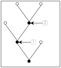
a is the number of steps it takes to reach abt from abt0.
If abt0 is the complete tree and abt is the subtree pointed to by the circled 1, the accumulator’s value must be 1 because it takes exactly one step to get from the root of abt to the root of abt0.
In the same spirit, for the subtree labeled 2 the accumulator is 2 because it takes two steps to get to this place.
(define (height.v2 abt0) (local (; Tree N -> N ; measures the height of abt ; accumulator a is the number of steps ; it takes to reach abt from abt0 (define (height/a abt a) (cond [(empty? abt) a] [else (... (height/a (node-left abt) (+ a 1)) ... ... (height/a (node-right abt) (+ a 1)) ...)]))) (height/a abt0 0)))
; Tree -> N ; measures the height of abt0 (check-expect (height.v2 example) 3) (define (height.v2 abt0) (local (; Tree N -> N ; measures the height of abt ; accumulator a is the number of steps ; it takes to reach abt from abt0 (define (height/a abt a) (cond [(empty? abt) a] [else (max (height/a (node-left abt) (+ a 1)) (height/a (node-right abt) (+ a 1)))]))) (height/a abt0 0)))
Following the design recipe also tells us that we need to interpret the two values to find the appropriate function. According to the purpose statement for height/a, the first value is the height of the left subtree, and the second one is the height of the right one. Given that we are interested in the height of abt itself and that the height is the largest number of steps it takes to reach a leaf, we use the max function to pick the proper one; see figure 185 for the complete definition.
The first accumulator, a, represents the number of steps it takes to reach abt from abt0, and the second accumulator stands for the tallest branch in the part of abt0 that is to the left of abt.
... ; Tree N N -> N ; measures the height of abt ; accumulator s is the number of steps ; it takes to reach abt from abt0 ; accumulator m is the maximal height of ; the part of abt0 that is to the left of abt (define (h/a abt s m) (cond [(empty? abt) ...] [else (... (h/a (node-left abt) ... s ... ... m ...) ... ... (h/a (node-right abt) ... s ... ... m ...) ...)])) ...
Exercise 498. Complete the design of height.v3. Hint In terms of the bottom-most tree of figure 184, the place marked 1 has no complete paths to leafs to its left while the place marked 2 has one complete path and it consists of two steps.
This second design has a more complex accumulator invariant than the first one. By implication, its implementation requires more care than the first one. At the same time, it comes without any advantages, meaning it is inferior to the first one.
Our point is that different accumulator invariants yield different variants. You can design both variants systematically, following the same design recipe. When you have complete function definitions, you can compare and contrast the results, and you can then decide which one to keep, based on evidence. End
Exercise 499. Design an accumulator-style version of product, the function that computes the product of a list of numbers. Stop when you have formulated the accumulator invariant and have someone check it.
The performance of product is O(n) where n is the length of the list. Does the accumulator version improve on this?
Exercise 500. Design an accumulator-style version of how-many, which is the function that determines the number of items on a list. Stop when you have formulated the invariant and have someone check it.
The performance of how-many is O(n) where n is the length of the list. Does the accumulator version improve on this?
Computer scientists refer to this space as stack space, but you can safely ignore this terminology for now.
When you evaluate (how-many some-non-empty-list) by hand, n
applications of add1 are pending by the time the function reaches
'()—
; N -> Number ; adds n to pi without using + (check-within (add-to-pi 2) (+ 2 pi) 0.001) (define (add-to-pi n) (cond [(zero? n) pi] [else (add1 (add-to-pi (sub1 n)))]))
Exercise 502. Design the function palindrome, which accepts a non-empty list and constructs a palindrome by mirroring the list around the last item. When given (explode "abc"), it yields (explode "abcba").
; [NEList-of 1String] -> [NEList-of 1String] ; creates a palindrome from s0 (check-expect (mirror (explode "abc")) (explode "abcba")) (define (mirror s0) (append (all-but-last s0) (list (last s0)) (reverse (all-but-last s0))))
via all-but-last,
via last,
via all-but-last again, and
via reverse, which is ISL+’s version of invert.
; Matrix -> Matrix ; finds a row that doesn't start with 0 and ; uses it as the first one ; generative moves the first row to last place ; no termination if all rows start with 0 (check-expect (rotate-until.v2 '((0 4 5) (1 2 3))) '((1 2 3) (0 4 5))) (define (rotate M) (cond [(not (= (first (first M)) 0)) M] [else (rotate (append (rest M) (list (first M))))]))
rows in M
1000
2000
3000
4000
5000
17
66
151
272
436
(define (rotate.v2 M0) (local (; Matrix ... -> Matrix ; accumulator ... (define (rotate/a M seen) (cond [(empty? M) ...] [else (... (rotate/a (rest M) ... seen ...) ...)]))) (rotate/a M0 ...)))
Formulate an accumulator statement. Then follow the accumulator design recipe to complete the above function. Measure how fast it runs on a Matrix that consists of rows with leading 0s except for the last one. If you completed the design correctly, the function is quite fast.
Exercise 504. Design to10. It consumes a list of digits and produces the corresponding number. The first item on the list is the most significant digit. Hence, when applied to '(1 0 2), it produces 102.
Domain Knowledge You may recall from grade school that the result is determined by
![]()
Exercise 505. Design the function is-prime, which consumes a natural number and returns #true if it is prime and #false otherwise.
Domain Knowledge A number n is prime if it is not divisible by any number between n - 1 and 2.
; N [>=1] -> Boolean ; determines whether n is a prime number (define (is-prime? n) (cond [(= n 1) ...] [else (... (is-prime? (sub1 n)) ...)]))
!.v1
5.760
5.780
5.800
5.820
5.870
5.806
!.v2
5.970
5.940
5.980
5.970
6.690
6.111
Exercise 506. Design an accumulator-style version of map.
(check-expect (f*ldl + 0 '(1 2 3)) (foldl + 0 '(1 2 3))) (check-expect (f*ldl cons '() '(a b c)) (foldl cons '() '(a b c))) ; version 1 (define (f*ldl f e l) (foldr f e (reverse l)))
; version 2 (define (f*ldl f e l) (local ((define (reverse l) (cond [(empty? l) '()] [else (add-to-end (first l) (reverse (rest l)))])) (define (add-to-end x l) (cond [(empty? l) (list x)] [else (cons (first l) (add-to-end x (rest l)))])) (define (foldr l) (cond [(empty? l) e] [else (f (first l) (foldr (rest l)))]))) (foldr (reverse l))))
; version 3 (define (f*ldl f e l) (local ((define (invert/a l a) (cond [(empty? l) a] [else (invert/a (rest l) (cons (first l) a))])) (define (foldr l) (cond [(empty? l) e] [else (f (first l) (foldr (rest l)))]))) (foldr (invert/a l '()))))
; version 4 (define (f*ldl f e l0) (local ((define (fold/a a l) (cond [(empty? l) a] [else (fold/a (f (first l) a) (rest l))]))) (fold/a e l0)))
; [X Y] [X Y -> Y] Y [List-of X] -> Y
(check-expect (build-l*st n f) (build-list n f))
32.4 A Graphical Editor, with Mouse
A Graphical Editor introduces the notion of a one-line editor and presents a number of exercises on creating a graphical editor. Recall that a graphical editor is an interactive program that interprets key events as editing actions on a string. In particular, when a user presses the left or right arrow keys, the cursor moves left or right; similarly, pressing the delete key removes a 1String from the edited text. The editor program uses a data representation that combines two strings in a structure. A Graphical Editor, Revisited resumes these exercises and shows how the same program can greatly benefit from a different data structure, one that combines two strings.
Neither of these sections deals with mouse actions for navigation, even though all modern applications support this functionality. The basic difficulty with mouse events is to place the cursor at the appropriate spot. Since the program deals with a single line of text, a mouse click at (x,y) clearly aims to place the cursor between the letters that are visible at or around the x position. This section fills the gap.
Recall the relevant definitions from A Graphical Editor, Revisited:
(define FONT-SIZE 11) (define FONT-COLOR "black") ; [List-of 1String] -> Image ; renders a string as an image for the editor (define (editor-text s) (text (implode s) FONT-SIZE FONT-COLOR)) (define-struct editor [pre post]) ; An Editor is a structure: ; (make-editor [List-of 1String] [List-of 1String]) ; interpretation if (make-editor p s) is the state of ; an interactive editor, (reverse p) corresponds to ; the text to the left of the cursor and s to the ; text on the right
(make-editor p s)
(string=? (string-append p s) ed)
(<= (image-width (editor-text p)) x (image-width (editor-text (append p (first s)))))
Hints (1) The x-coordinate measures the distance from the left. Hence the function must check whether smaller and smaller prefixes of ed fit into the given width. The first one that doesn’t fit corresponds to the pre field of the desired Editor, the remainder of ed to the post field.
(2) Designing this function calls for thoroughly developing examples and tests. See Intervals, Enumerations, and Itemizations.
Exercise 509. Design the function split. Use the accumulator design recipe to improve on the result of exercise 508. After all, the hints already point out that when the function discovers the correct split point, it needs both parts of the list, and one part is obviously lost due to recursion.
Once you have solved this exercise, equip the main function of
A Graphical Editor, Revisited with a clause for mouse
clicks. As you experiment with moving the cursor via mouse clicks, you will
notice that it does not exactly behave like applications that you use on
your other devices—
Graphical programs, like editors, call for experimentation to come up with the best “look and feel” experiences. In this case, your editor is too simplistic with its placement of the cursor. After the applications on your computer determine the split point, they also determine which letter division is closer to the x-coordinate and place the cursor there.
Exercise 510. Many operating systems come with the fmt program, which can rearrange the words in a file so that all lines in the resulting file have a maximal width. As a widely used program, fmt supports a range of related functions. This exercise focuses on its core functionality.
Design the program fmt. It consumes a natural number w,
the name of an input file in-f, and the name of an output file
out-f—
33 More Uses of Accumulation
This chapter presents three more uses of accumulators. The first section concerns the use of accumulators in conjunction with tree-processing functions. It uses the compilation of ISL+ as an illustrative example. The second section explains why we occasionally want accumulators inside of data representations and how to go about placing them there. The final section resumes the discussion of rendering fractals.
33.1 Accumulators and Trees
When you ask DrRacket to run an ISL+ program, it translates the program to commands for your specific computer. This process is called compilation, and the part of DrRacket that performs the task is called a compiler. Before the compiler translates the ISL+ program, it checks that every variable is declared via a define, a define-struct, or a lambda.
Stop! Enter x, (lambda (y) x), and (x 5) as complete ISL+ programs into DrRacket and ask it to run each. What do you expect to see?
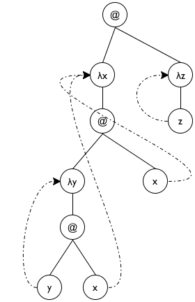
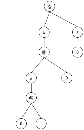
Sample Problem You have been hired to re-create a part of the ISL+ compiler. Specifically, your task deals with the following language fragment, specified in the so-called grammar notation that many programming language manuals use:We use the Greek letter λ instead of lambda to signal that this exercise deals with ISL+ as an object of study, not just a programming language.
expression = variable | (λ (variable) expression) | (expression expression) Remember from intermezzo 1 that you can read the grammar aloud replacing = with “is one of” and | with “or.”Recall that λ expressions are functions without names. They bind their parameter in their body. Conversely, a variable occurrence is declared by a surrounding λ that specifies the same name as a parameter. You may wish to revisit Intermezzo 3: Scope and Abstraction because it deals with the same issue from the perspective of a programmer. Look for the terms “binding occurrence,” “bound occurrence,” and “free.”
Develop a data representation for the above language fragment; use symbols to represent variables. Then design a function that replaces all undeclared variables with '*undeclared.
(λ (x) x) is the function that returns whatever it is given, also known as the identity function;
(λ (x) y) looks like a function that returns y whenever it is given an argument, except that y isn’t declared;
(λ (y) (λ (x) y)) is a function that, when given some value v, produces a function that always returns v;
((λ (x) x) (λ (x) x)) applies the identity function to itself;
(((λ (y) (λ (x) y)) (λ (z) z)) (λ (w) w)) is a complex expression that is best run in ISL+ to find out whether it terminates.
Exercise 511. Explain the scope of each binding occurrence in the above examples. Draw arrows from the bound to the binding occurrences.
(define ex1 '(λ (x) x)) (define ex2 '(λ (x) y)) (define ex3 '(λ (y) (λ (x) y))) (define ex4 '((λ (x) (x x)) (λ (x) (x x))))
Exercise 512. Define is-var?, is-λ?, and is-app?, that is, predicates that distinguish variables from λ expressions and applications.
λ-para, which extracts the parameter from a λ expression;
λ-body, which extracts the body from a λ expression;
app-fun, which extracts the function from an application; and
app-arg, which extracts the argument from an application.
Design declareds, which produces the list of all symbols used as λ parameters in a λ term. Don’t worry about duplicate symbols.
Exercise 513. Develop a data representation for the same subset of ISL+ that uses structures instead of lists. Also provide data representations for ex1, ex2, and ex3 following your data definition.
; Lam -> Lam ; replaces all symbols s in le with '*undeclared ; if they do not occur within the body of a λ ; expression whose parameter is s (check-expect (undeclareds ex1) ex1) (check-expect (undeclareds ex2) '(λ (x) *undeclared)) (check-expect (undeclareds ex3) ex3) (check-expect (undeclareds ex4) ex4) (define (undeclareds le0) le0)
(define (undeclareds le) (cond [(is-var? le) ...] [(is-λ? le) (... (undeclareds (λ-body le)) ...)] [(is-app? le) (... (undeclareds (app-fun le)) ... (undeclareds (app-arg le)) ...)]))
(define (undeclareds le0) (local (; Lam ??? -> Lam ; accumulator a represents ... (define (undeclareds/a le a) (cond [(is-var? le) ...] [(is-λ? le) (... (undeclareds/a (λ-body le) ... a ...) ...)] [(is-app? le) (... (undeclareds/a (app-fun le) ... a ...) ... (undeclareds/a (app-arg le) ... a ...) ...)]))) (undeclareds/a le0 ...)))
a represents the list of λ parameters encountered on the path from the top of le0 to the top of le.
'(((λ (y) (λ (x) y)) (λ (z) z)) (λ (w) w))
'(((λ (y) (λ (x) y)) (λ (z) z)) (λ (w) w))
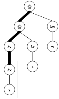
Figure 186: Lam terms as trees
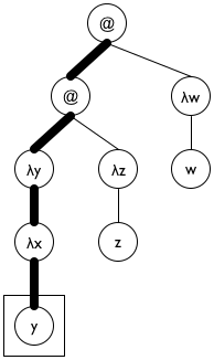
We pick an initial accumulator value of '().
We use cons to add (λ-para le) to a.
We exploit the accumulator for the clause where undeclareds/a deals with a variable. Specifically, the function uses the accumulator to check whether the variable is in the scope of a declaration.
Figure 187 shows how to translate these ideas into a complete function definition. Note the name declareds for the accumulator; it brings across the key idea behind the accumulator invariant, helping the programmer understand the definition. The base case uses member? from ISL+ to determine whether the variable le is in declareds and, if not, replaces it with '*undeclared. The second cond clause uses a local to introduce the extended accumulator newd. Because para is also used to rebuild the expression, it has its own local definition. Finally, the last clause concerns function applications, which do not declare variables and do not use any directly. As a result, it is by far the simplest of the three clauses.
; Lam -> Lam (define (undeclareds le0) (local (; Lam [List-of Symbol] -> Lam ; accumulator declareds is a list of all λ ; parameters on the path from le0 to le (define (undeclareds/a le declareds) (cond [(is-var? le) (if (member? le declareds) le '*undeclared)] [(is-λ? le) (local ((define para (λ-para le)) (define body (λ-body le)) (define newd (cons para declareds))) (list 'λ (list para) (undeclareds/a body newd)))] [(is-app? le) (local ((define fun (app-fun le)) (define arg (app-arg le))) (list (undeclareds/a fun declareds) (undeclareds/a arg declareds)))]))) (undeclareds/a le0 '())))
Exercise 514. Make up an ISL+ expression in which x occurs both free and bound. Formulate it as an element of Lam. Does undeclareds work properly on your expression?
(list '*undeclared 'x)
(list '*declared 'y)
Note The trick of replacing a variable occurrence with the representation of an application feels awkward. If you dislike it, consider synthesizing the symbols '*undeclared:x and 'declared:y instead.
Exercise 516. Redesign the undeclareds function for the structure-based data representation from exercise 513.
'((λ (x) ((λ (y) (y x)) x)) (λ (z) z))
Hint The undeclareds accumulator of undeclareds/a
is a list of all parameters on path from le to le0
in reverse order—
33.2 Data Representations with Accumulators
The end of Intermezzo 5: The Cost of Computation explains that *SL measures the size of containers, say lists, by traversing them and hints that other programming languages use a different,See Finite State Machines for an early example of this idea. less expensive way, to compute sizes. In this section, we show how to implement this idea with the addition of an accumulator to data representations.
Consider the ubiquitous lists in *SL. All lists are constructed from cons and '(); operations such as quote and list, for example, are merely abbreviations for these two. As What Is '(), What Is cons shows, it is also possible to mimic lists in BSL with suitable structure type and function definitions.
(define-struct pair [left right]) ; ConsOrEmpty is one of: ; – '() ; – (make-pair Any ConsOrEmpty) ; Any ConsOrEmpty -> ConsOrEmpty (define (our-cons a-value a-list) (cond [(empty? a-list) (make-pair a-value a-list)] [(our-cons? a-list) (make-pair a-value a-list)] [else (error "our-cons: ...")])) ; ConsOrEmpty -> Any ; extracts the left part of the given pair (define (our-first mimicked-list) (if (empty? mimicked-list) (error "our-first: ...") (pair-left mimicked-list)))
Figure 189 recalls the basic idea. Stop! Can you define our-rest now?
(define-struct cpair [count left right]) ; A [MyList X] is one of: ; – '() ; – (make-cpair (tech "N") X [MyList X]) ; accumulator the count field is the number of cpairs
; data definitions, via a constructor-function (define (our-cons f r) (cond [(empty? r) (make-cpair 1 f r)] [(cpair? r) (make-cpair (+ (cpair-count r) 1) f r)] [else (error "our-cons: ...")]))
; Any -> N ; how many items does l contain (define (our-length l) (cond [(empty? l) 0] [(cpair? l) (cpair-count l)] [else (error "my-length: ...")]))
The second problem with the addition of a count field concerns
performance. Indeed, there are two concerns. On the one hand, every single
list construction comes with an extra field now, meaning a 33% increase in
memory consumption. On the other hand, the addition of the field decreases
how fast our-cons constructs a list. In addition to the check
that the extended list is either '() or an instance of a cpair,
the constructor now computes the size of the list. Although this
computation consumes a constant amount of time, it is imposed on every
single use of our-cons—
Exercise 518. Argue that our-cons takes a constant amount of time to compute its result, regardless of the size of its input.
Exercise 519. Is it acceptable to impose the extra cost on cons for all programs to turn length into a constant-time function?
While the addition of a count field to lists is questionable, sometimes data accumulators play a crucial role in finding a solution. The next example is about adding so-called artificial intelligence to a board-game-playing program, and its data accumulator is an absolute necessity.
Sample Problem Your manager tells you the following story.
“Once upon a time, three cannibals were guiding three missionaries through a jungle. They were on their way to the nearest mission station. After some time, they arrived at a wide river, filled with deadly snakes and fish. There was no way to cross the river without a boat. Fortunately, they found a rowboat with two oars after a short search. Unfortunately, the boat was too small to carry all of them. It could barely carry two people at a time. Worse, because of the river’s width someone had to row the boat back.
“Since the missionaries could not trust the cannibals, they had to figure out a plan to get all six of them safely across the river. The problem was that these cannibals would kill and eat missionaries as soon as there were more cannibals than missionaries in some place. Our missionaries had to devise a plan that guaranteed that there were never any missionaries in the minority on either side of the river. The cannibals, however, could be trusted to cooperate otherwise. Specifically, they would not abandon any potential food, just as the missionaries would not abandon any potential converts.”
While your manager doesn’t assign any specific design task, he wants to explore whether the company can design (and sell) programs that solve such puzzles.
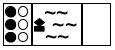
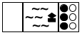
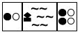
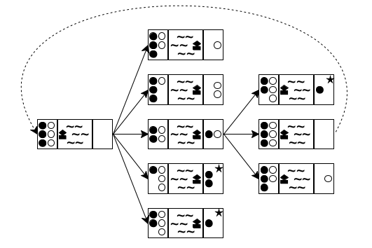
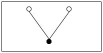
Now that you have a way to write down the state of the puzzle, you can think about the possibilities at each stage. Doing so yields a tree of possible moves. Figure 190 sketches the first two and a half layers in such a tree. The left-most state is the initial one. Because the boat can transport at most two people and must be rowed by at least one, you have five possibilities to explore: one cannibal rows across; two cannibals row across; one missionary and one cannibal go; one missionary crosses; or two missionaries do. These possibilities are represented with five arrows going from the initial state to five intermediate states.
For each of these five intermediate states, you can play the same game again. In figure 190 you see how the game continues for the middle (third) one of the new states. Because there are only two people on the right river bank, you see three possibilities: a cannibal goes back, a missionary goes back, or both do. Hence three arrows connect the middle state to the three states on the right side of the tree. If you keep drawing this tree of possibilities in a systematic manner, you eventually discover the final state.
A second look at figure 190 reveals two problems with this naive approach to generating the tree of possibilities. The first one is the dashed arrow that connects the middle state on the right to the initial state. It indicates that rowing back the two people from the right to the left gets the puzzle back to its initial state, meaning you’re starting over, which is obviously undesirable. The second problem concerns those states with a star in the top-right corner. In both cases, there are more white-circle cannibals than black-circle missionaries on the left river bank, meaning the cannibals would eat the missionaries. Again, the goal is to avoid such states, making these moves undesirable.
; PuzzleState -> PuzzleState ; is the final state reachable from state0 ; generative creates a tree of possible boat rides ; termination ??? (check-expect (solve initial-puzzle) final-puzzle) (define (solve state0) (local (; [List-of PuzzleState] -> PuzzleState ; generative generates the successors of los (define (solve* los) (cond [(ormap final? los) (first (filter final? los))] [else (solve* (create-next-states los))]))) (solve* (list state0))))
Clearly, solve is quite generic. As long as you define a collection of PuzzleStates, a function for recognizing final states, and a function for creating all “successor” states, solve can work on your puzzle.
Exercise 520. The solve* function generates all states reachable with n boat trips before it looks at states that require n + 1 boat trips, even if some of those boat trips return to previously encountered states. Because of this systematic way of traversing the tree, solve* cannot go into an infinite loop. Why? Terminology This way of searching a tree or a graph is dubbed breadth-first search.
Exercise 521. Develop a representation for the states of the missionary-and-cannibal puzzle. Like the graphical representation, a data representation must record the number of missionaries and cannibals on each side of the river plus the location of the boat.
The description of PuzzleState calls for a new structure type. Represent the above initial, intermediate, and final states in your representation.
Design the function final?, which detects whether in a given state all people are on the right river bank.
Design the function render-mc, which maps a state of the missionary-and-cannibal puzzle to an image.
The problem is that returning the final state says nothing about how the player can get from the initial state to the final one. In other words, create-next-states forgets how it gets to the returned states from the given ones. And this situation clearly calls for an accumulator, but at the same time, the accumulated knowledge is best associated with every individual PuzzleState, not solve* or any other function.
Exercise 522. Modify the representation from exercise 521 so that a state records the sequence of states traversed to get there. Use a list of states.
Articulate and write down an accumulator statement with the data definition that explains the additional field.
Modify final? or render-mc for this representation as needed.
Exercise 523. Design the create-next-states function. It consumes lists of missionary-and-cannibal states and generates the list of all those states that a boat ride can reach.
Ignore the accumulator in the first draft of create-next-states, but make sure that the function does not generate states where the cannibals can eat the missionaries.
For the second design, update the accumulator field in the state structures and use it to rule out states that have been encountered on the way to the current state.
Exercise 524. Exploit the accumulator-oriented data representation to modify solve. The revised function produces the list of states that lead from the initial PuzzleState to the final one.
Also consider creating a movie from this list, using render-mc to generate the images. Use run-movie to display the movie.
33.3 Accumulators as Results
The given problem is a triangle. When the triangle is too small to be subdivided any further, the algorithm does nothing; otherwise, it finds the midpoints of its three sides and deals with the three outer triangles recursively.
Sample Problem Design the add-sierpinski function. It consumes an image and three Posns describing a triangle. It uses the latter to add a Sierpinski triangle to this image.
The problem is trivial if the triangle is too small to be subdivided.
In the trivial case, the function returns the given image.
Otherwise the midpoints of the sides of the given triangle are determined to add another triangle. Each “outer” triangle is then processed recursively.
Each of these recursive steps produces an image. The remaining question is how to combine these images.
; Image Posn Posn Posn -> Image ; generative adds the triangle (a, b, c) to s, ; subdivides it into three triangles by taking the ; midpoints of its sides; stop if (a, b, c) is too small (define (add-sierpinski scene0 a b c) (cond [(too-small? a b c) scene0] [else (local ((define scene1 (add-triangle scene0 a b c)) (define mid-a-b (mid-point a b)) (define mid-b-c (mid-point b c)) (define mid-c-a (mid-point c a)) (define scene2 (add-sierpinski scene0 a mid-a-b mid-c-a)) (define scene3 (add-sierpinski scene0 b mid-b-c mid-a-b)) (define scene4 (add-sierpinski scene0 c mid-c-a mid-b-c))) ; — IN— (... scene1 ... scene2 ... scene3 ...))])) Figure 191: Accumulators as results of generative recursions, a skeleton
Figure 191 shows the result of translating these answers into a skeletal definition. Since each midpoint is used twice, the skeleton uses local to formulate the generative step in ISL+. The local expression introduces the three new midpoints plus three recursive applications of add-sierpinski. The dots in its body suggest a combination of the scenes.
; Image Posn Posn Posn -> Image ; adds the black triangle a, b, c to scene (define (add-triangle scene a b c) scene) ; Posn Posn Posn -> Boolean ; is the triangle a, b, c too small to be divided (define (too-small? a b c) #false) ; Posn Posn -> Posn ; determines the midpoint between a and b (define (mid-point a b) a)
Now that we have all the auxiliary functions, it is time to return to the problem of combining the three images that are created by the recursive calls. One obvious guess is to use the overlay or underlay function, but an evaluation in the interactions area of DrRacket shows that the functions hide the underlying triangles.
> scene1
> scene2
> scene3
; Image Posn Posn Posn -> Image ; generative adds the triangle (a, b, c) to s, ; subdivides it into three triangles by taking the ; midpoints of its sides; stop if (a, b, c) is too small ; accumulator the function accumulates the triangles scene0 (define (add-sierpinski scene0 a b c) (cond [(too-small? a b c) scene0] [else (local ((define scene1 (add-triangle scene0 a b c)) (define mid-a-b (mid-point a b)) (define mid-b-c (mid-point b c)) (define mid-c-a (mid-point c a)) (define scene2 (add-sierpinski scene1 a mid-a-b mid-c-a)) (define scene3 (add-sierpinski scene2 b mid-b-c mid-a-b))) ; — IN— (add-sierpinski scene3 c mid-c-a mid-b-c))])) Figure 192: Accumulators as results of generative recursion, the function
Figure 192 shows the reformulation based on this insight. The three highlights pinpoint the key design idea. All concern the case when the triangle is sufficiently large and it is added to the given scene. Once its sides are subdivided, the first outer triangle is recursively processed using scene1, the result of adding the given triangle. Similarly, the result of this first recursion, dubbed scene2, is used for the second recursion, which is about processing the second triangle. Finally, scene3 flows into the third recursive call. In sum, the novelty is that the accumulator is simultaneously an argument, a tool for collecting knowledge, and the result of the function.
(define MT (empty-scene 400 400)) (define A (make-posn 200 50)) (define B (make-posn 27 350)) (define C (make-posn 373 350)) (add-sierpinski MT A B C)
Exercise 526. To compute the endpoints of an equilateral Sierpinski triangle, draw a circle and pick three points on the circle that are 120 degrees apart, for example, 120, 240, and 360.
(define CENTER (make-posn 200 200)) (define RADIUS 200) ; the radius in pixels ; Number -> Posn ; determines the point on the circle with CENTER ; and RADIUS whose angle is ; examples ; what are the x and y coordinates of the desired ; point, when given: 120/360, 240/360, 360/360 (define (circle-pt factor) (make-posn 0 0))
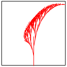
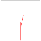
Design the function add-savannah. The function consumes an image and four numbers: (1) the x-coordinate of a line’s base point, (2) the y-coordinate of a line’s base point, (3) the length of the line, and (4) the angle of the line. It adds a fractal Savannah tree to the given image.
Unless the line is too short, the function adds the specified line to the image. It then divides the line into three segments. It recursively uses the two intermediate points as the new starting points for two lines. The lengths and the angles of the two branches change in a fixed manner, but independently of each other. Use constants to define these changes and work with them until you like your tree well enough.
Hint Experiment with shortening each left branch by at least one third and rotating it left by at least 0.15 degrees. For each right branch, shorten it by at least 20% and rotate it by 0.2 degrees in the opposite direction.
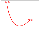
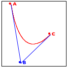
Now turn to the image in the middle. It explains the essential idea of the generative step. The algorithm determines the midpoint on the two observer lines, A-B and B-C, as well as their midpoint, A-B-C.
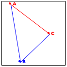
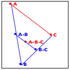
Finally, the right-most image shows how these three new points generate two distinct recursive calls: one deals with the new triangle on the left and the other one with the triangle on the right. More precisely, A-B and B-C become the new observer points and the lines from A to A-B-C and from C to A-B-C become the foci of the two recursive calls.
When the triangle is small enough, we have a trivially solvable case. The algorithm just draws the triangle, and it appears as a point on the given image. As you implement this algorithm, you need to experiment with the notion of “small enough” to make the curve look smooth.
34 Summary
The first step is to recognize the need for introducing an accumulator. Traversals “forget” pieces of the argument when they step from one piece to the next. If you discover that such knowledge could simplify the function’s design, consider introducing an accumulator. The first step is to switch to the accumulator template.
The key step is to formulate an accumulator statement. The latter must express what knowledge the accumulator gathers as what kind of data. In most cases, the accumulator statement describes the difference between the original argument and the current one.
The third step, a minor one, is to deduce from the accumulator statement (a) what the initial accumulator value is, (b) how to maintain it during traversal steps, and (c) how to exploit its knowledge.
The idea of accumulating knowledge is ubiquitous, and it appears in many different forms and shapes. It is widely used in so-called functional languages like ISL+. Programmers using imperative languages encounter accumulators in a different way, mostly via assignment statements in primitive looping constructs because the latter cannot return values. Designing such imperative accumulator programs proceeds just like the design of accumulator functions here, but the details are beyond the scope of this first book on systematic program design.